Before all, if you’ve ever heard of hierarchical modeling (HLM), multilevel modeling (MLM), or mixed-effects model…they all mean the same thing! I hope people don’t get too confused by the messy terms.
Why HLM?
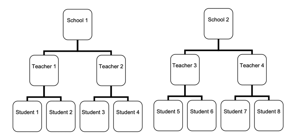
In practice, data are often not randomly distributed. For example, students attend different schools and are taught by different math teachers within those schools. This creates a nested structure in our data — students within teachers, and teachers within schools (see Fig 1).1
If you’re familiar with regression models, you might notice that our data violate the assumption of independence. In other words, the data are clustered. Ignoring this nesting structure and running a standard statistical test can bias the results. Students within the same group are not truly independent—they share similarities that make them more alike than students from different groups. Treating them as independent effectively inflates the sample size and underestimates the standard errors, which increases the risk of a Type I error. In short, even if a test appears significant, the result may not actually be significant at all.
You might be wondering, “Why not just remove those levels?” Indeed, we could take the average for each school, for example. By collapsing across teachers and students, we would reduce the data from 3 levels to 1. However, this approach decreases the sample size, which in turn reduces statistical power and increases the likelihood of a Type II error. In other words, a real effect might exist, but we could fail to detect it in our analysis.
In addition, ignoring the nesting structure could result in two conceptual errors: ecological fallacy and atomistic fallacy. Ecological fallacy means that your conclusion is about individuals (e.g., students), but it’s made based on group analysis (e.g., schools). Atomistic fallacy is that your conclusion is about the group, but it’s made based on individual analysis.
Why is this problematic? Imagine our results show that schools with a more positive climate tend to host more sports events each year. If we then conclude that students in positive-climate schools are more likely to participate in sports, we would be committing an ecological fallacy—assuming that relationships observed at the group level also apply to individuals. In reality, some students in those schools might not participate in sports at all.
Likewise, suppose we find that students with higher self-efficacy tend to have higher math scores. If we then infer that schools with more confident students achieve higher overall math performance, we would commit an atomistic fallacy—generalizing individual-level relationships to the group level.
In short, relationships at one level of analysis do not automatically transfer to another. Ignoring the nested structure of data can lead to one or both of these fallacies, as we mistakenly attribute individual behaviors to groups or group characteristics to individuals.
Random Intercept Model (2-level)
We use HLM to deal with non-independent observations. In short, HLM has two components: random effects and fixed effects. A slope and an intercept can either be random or fixed. Random effects vary across groups. Fixed effects is fixed in the population.
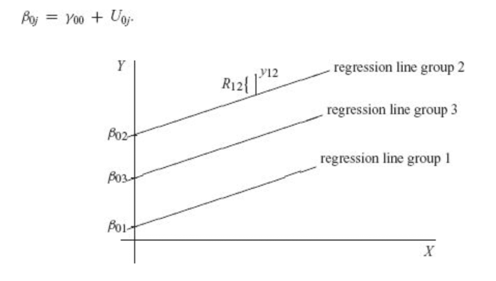
In a simple linear regression, both slope and intercept are fixed. In HLM, we can either 1) set a random intercept or 2) set both random intercept and random slope. We typically don’t do random slopes alone. It may help if we look at Fig 2.2 We see parallel regression lines, each is for a group, cluster, or level, whatever we prefer to call. Intercept varies across groups, and the slope stays fixed. The figure shows the simplest form of HLM: random intercept model (RIM).
RIM has a random intercept and a fixed slope. In this example, our RIM incorporates two levels of data. Level 1 is about individual students. Level 2 is about schools. RIM captures the deviation of group means from the population grand mean. Let’s look at the null model:3
$$
\text{Level 1: } Y_{ij} = \beta_{0j} + r_{ij} \text{ , } r_{ij} \sim N(0, \sigma^2)
$$
$$
\text{Level 2: } \beta_{0j} = \gamma_{00} + u_{0j} \text{ , } u_{0j} \sim N(0, \tau_0^2)
$$
or if we combine the terms together,
$$
Y_{ij} = \gamma_{00} + u_{0j} + r_{ij} \text{ , } r_{ij} \sim N(0, \sigma^2) \text{ , } u_{0j} \sim N(0, \tau_0^2)
$$
where
- $i=(1…n_j)$ denotes the individual index for each group; $j=(1…J)$ denotes the group index.
- $\beta_{0j}$ is the average outcome for the $j$th group.
- $\gamma_{00}$ is the population grand mean; fixed intercept.
- $u_{0j}$ is the random deviation of group mean for the $j$th group from the population grand mean $(\gamma_{00})$; random intercept.
- $\tau_0^2$ is the between-group variance for level 2, indicating the variance of group means $(\beta_{0j})$.
- $r_{ij}$ is the residual of individual $i$ in group $j$.
- $\sigma^2$ is the within-group variance and is at level 1.
We can think of this as schools having different average math scores at baseline. Each school mean fluctuates around the population mean by $u_{0j}$. We capture the variance of that fluctuation, $\tau_0^2$ , to estimate the effect of schools on math scores. By summing $u_{0j}$ and population grand mean $(\gamma_{00})$, we get the random intercept $\beta_{0j}$ that varies across groups. Lastly, we add the $r_{ij}$ , the residual for each individual.
So, we have 3 RIM parameters to estimate: $\gamma_{00}$, $\tau_0^2$, and $\sigma^2$. Each key parameter represents a question of potential interest:
- $\gamma_{00}$: What do we know about the average math score for the population?
- $\tau_0^2$: How do math scores vary by schools?
- $\sigma^2$: How do math scores vary by students?
Similarly, for RIM with predictor $x$, it can be written as:
$$
\text{Level 1: } Y_{ij} = \beta_{0j} + \beta_{1j}x_{ij} + r_{ij} \text{ , } r_{ij} \sim N(0, \sigma^2)
$$
$$
\text{Level 2: } \beta_{0j} = \gamma_{00} + u_{0j} \text{ , } u_{0j} \sim N(0, \tau_0^2) \text{ ; } \beta_{1j} = \gamma_{10}
$$
or equivalently,
$$
Y_{ij} = \gamma_{00} + \gamma_{10}x_{ij} + u_{0j} + r_{ij} \text{ , } r_{ij} \sim N(0, \sigma^2) \text{ , } u_{0j} \sim N(0, \tau_0^2)
$$
where the new term $\gamma_{10}$ is the fixed slope between $Y_{ij}$ and $x_{ij}$. It’s shared by all groups. By fixing the slope, we assume that 1-unit increase in $x_{ij}$ have the same effect on the increase in students’ math scores for each school. Nothing new going on here. The intercept still varies, and the slope of $x$ is fixed for all schools.
For the model above, we have the following assumptions:
- Linear relationship between $Y_{ij}$ and $x_{ij}$
- $u_{0j}$ $\perp$ $r_{ij}$ ; $r_{ij}$ $\perp$ $r_{i’j}$ , where $i$ ≠ $i’$
- $u_{0j}$ is independent across schools
These assumptions are useful because they will help us calculate and interpret intraclass correlation, which I will discuss in the next section.
Intraclass Correlation
To check whether to use an HLM on your data, we estimate the intraclass correlation (ICC). If ICC is high enough (based on the criteria in your field), that indicates sufficient group-level variance compared to the total variance. Then, we choose to use HLM.
ICC ranges from 0 to 1. If ICC is super high, it means that the variance is entirely due to schools, instead of individual differences in students. If ICC is super low, we can ignore the school effect and give up HLM — just fit a simple linear regression instead. Different fields have different consensus for a large ICC. In education, ICC of 0.2 can be high enough to suggest a multilevel structure, but this may not be enough in other fields.
Generally, ICC has two interpretations:
- The proportion of variance accounted by groups.
- e.g., 28% of the variance is accounted for by the school students attend.
- The correlation between outcomes of two randomly selected individuals in the same randomly selected group.
- e.g., for two students attending the same school, the correlation between their math scores is 0.28.
In a two-level context, if we see ICC as the proportion of between-school variance, it can be written as:
$$
\text{ICC} = \frac{\text{between-group variance}}{\text{total variance}} = \frac{\text{Var}(u_{0j})}{\text{Var}(u_{0j}+r_{ij})} = \frac{\tau_0^2}{\tau_0^2 + \sigma^2}
$$
If we see ICC as how resemble two students from the same school are, we can write:
$$
\rho(Y_{ij},Y_{i’j}) = \frac{\text{Cov}(Y_{ij},Y_{i’j})}{\text{SD}(Y_{ij})\text{SD}(Y_{i’j})} = \frac{\text{Cov}(u_{0j}+r_{ij}, u_{0j}+r_{i’j})}{\sqrt{\text{Var}(u_{0j}+r_{ij})}\sqrt{\text{Var}(u_{0j}+r_{i’j})}} =\frac{\text{Cov}(u_{0j}, u_{0j})}{\sqrt{\tau_0^2 + \sigma^2} + \sqrt{\tau_0^2 + \sigma^2}}=\frac{\tau_0^2}{\tau_0^2 + \sigma^2}
$$
Let’s recall the assumptions of HLM. Since $r_{ij}$ is independent, and $u_{0j}$ and $r_{ij}$ are independent from each other, the covariance among $u_{0j}$, $r_{ij}$, and $r_{i’j}$ is all 0. We disregarded them when calculating $\text{Cov}(Y_{ij},Y_{i’j})$. Thus, the covariance between two students from the same school is $\text{Var}(u_{0j})$, the between-school variance. Both interpretations of ICC are correct. You can choose which one to use based on your research question.
Model Comparisons
After knowing if the data is multilevel, we still don’t know whether the multilevel structure matters in analysis. A simple model is always more preferable than a complex one. Hypothesis testing helps us see whether it’s worthy to keep random intercepts in our model. The null hypothesis is that the between-school variance is 0. The alternative hypothesis is that the between-school variance is greater than 0. In symbols, it writes as:
$$
H_0: \tau_0^2=0 \text{ , } H_a: \tau_0^2 > 0
$$
Essentially, we are wondering: is school randomness ($\tau_0^2$) large enough that we can use it to predict school means ($\beta_{0j}$)? If $\tau_0^2$ is close to 0 or when the sample size is large, we can just use the grand mean ($\gamma_{00}$) to predict school means. There is no need to fit an HLM! However, if $\tau_0^2$ is large enough, it will help us predict each school mean. Grand mean is no longer reliable since schools vary much from each other.
We can compare our RIM null model to a simple linear regression model by doing a likelihood ratio test (LRT). Some fields use maximum likelihood estimates, but statisticians minimize things just to be safe. So, we look at a model’s deviance, defined as $D=-2log \mathcal{L}$ , where $\mathcal{L}$ is the likelihood. In human words, deviance is “how bad the model fits”. So, we prefer models with a lower $D$ (badness).
$$
\text{LRT statistic} = -2log\frac{\mathcal{L}(\text{reduced})}{\mathcal{L}(\text{full})} = -2[log\mathcal{L}(\text{reduced}) – \mathcal{L}(\text{full})] = D_r – D_f \sim \chi_{df}
$$
As shown by the Eq above, likelihood of full model is subtracted from the reduced model, ending up with a $\chi^2$ statistic. It means we check whether there is a difference in badness between the simpler model and the more complex model. If the result is significant, we choose the more complex model (i.e., the RIM). In R, simply by running ranova(your_RIM), you will get useful info (AIC, $\chi^2$, p-values, etc.) for hypothesis testing of variance component.
Similarly, we can also choose the best fit model from RIMs with different predictors using LRT. The procedure is essentially the same. In R, it’s as simple as running anova(RIM1, RIM2, RIM3) . If these models are no different, then we keep the simple model — RIM with less predictors.
In future posts, I will talk about random slope models and 3-level models. The equations and interpretations will be very ugly (I cried when I learned it the first time), but I’ll try my best to explain things more intuitively. Thanks for reading.
- Noell, G.H., Porter, B.A., & Patt, M.J. (2007). Value Added Assessment of Teacher Preparation in Louisiana: 2004 – 2006. ↩︎
- Snijders, T. A. B., & Bosker, R. J. (2012). Multilevel analysis: An introduction to basic and advanced multilevel modeling(2. ed). SAGE. ↩︎
- a.k.a. empty model or unconditional model — a default model with no additional predictors. ↩︎